Astronomy · computer · Note

Least-Squares Fitting of data containing errors

(This is a note personal only! )

There is a powerful tool dealing with data containing both “X” and “Y” errors to make a lease-square fitting in IDL, that is mpfit. This routine allows you to use a self-defined function to do the fitting. Also, you can set up some conditions such as the parameters’ limit or fixed parameters etc. This is fabulous! So beginning with the actual astronomical data have errors both in “X” and “Y”, you need to use a function called “linfitex” (you can see more info from the mpfit website) to both define the function you want to fit and calculate the least-square needed in the fitting. Here is an example of the function:

FUCNTION myfunct, p, x=x, y=y \$
     , sigma_x=sigma_x, sigma_y=sigma_y, _EXTRA=extra
  a = p[0]
  b = p[1]
  f = a*alog10(X)+b
;#########calculate the derivative of the function#########
;##put into resid as (y-f)/sqrt(sigma_y^2+(y'*sigma_x)^2)## 
  resid = (y - f)/sqrt(sigma_y^2 + (a/(x*alog(10))*sigma_x)^2) 
RETURN, resid

In the code above I just defined a function as

    \[y=a \log_{10} (b)+c\]

Then you can read your data. and when you want to fit the data, just using mpfit as:

p      = [1,1,1]
p[1]   = 1         
p[2]   = 2
p[3]   = 3 ;initial guess of the parameters
param  = MPFIT('MYFUNCT', params,\$
      FUNCTARGS={X:x,Y:y,SIGMA_X:x_er,SIGMA_Y:y_er}, PERROR=p_er)

The FUNCTARGS is the place where your data go into the function. And then you can find the results of the parameters from the fitting by print “param” and also the 1σ error from printing p_er. If you only have the error on “Y”, you can use a function like this:

FUNCTION myfunct, p, x=x, y=y, er=er
  a = p[0]     
  b = p[1]
  c = p[2]
  f = a*alog10(b)+c
RETURN, (y-f)/er
END

And then using the same way described above to call “mpfit” and get the results and errors.

Here is also a PYTHON version of this procedure.
Astronomy · Note

A digest of arXiv:1112.0285

From: Evolution of Galaxy Formation, by Douglas Scott

From a view of the logic flow of the discovery of galaxy formation, we can learn that there are some important findings that have already exist before. Due to some reasons, maybe the depth of the research or the instrument limitation etc, when people revisit the topic after many years they can still find something new and make great discoveries. That means there are some potentially good stories hide in the old topics, maybe. So that shows us a good chance and direction from a historical view.

Also, the author makes some many possible future aspects of the subject on galaxy formation:

  • galaxy formation will not be completely “solved” in the near future;
  • ambitious multi-wavelength surveys will extend our empirical understanding of the high-z Universe; (this is really one of the hottest fields within the study of a galaxy)
  • there will continue to be phrases spun to describe new ideas;
  • some of these ideas will be old ideas, dressed up;(But I think this is not a bad thing)
  • some ideas will be crazy, and will fall by the wayside;
  • some ideas will genuinely progress the field, inspiring a new generation of galaxy fabricators;(So, big bosses dig holes and we fill them up)
Astronomy · Linux · Note

pgplot quick install guide

Here you can follow the steps to install pgplot on you linux OS.
First, you need to be sure you have X11 lib development packages installed, and then just follow the steps copied as below:

su
cd /usr/local/src
wget  ftp://ftp.astro.caltech.edu/pub/pgplot/pgplot5.2.tar.gz
tar -zxvf pgplot5.2.tar.gz
cd pgplot
mkdir /usr/local/pgplot
cd !$
cp /usr/local/src/pgplot/drivers.list .

then use vim to edit drivers.list in the directory, choose the PSDRIV 1,2,3,4 for EPS figures and XWDRIV 1,2 for X-window output. And then

/usr/local/src/pgplot/makemake /usr/local/src/pgplot linux g77_gcc
ln -s /usr/bin/g77-3.3 /usr/bin/g77 
#(if you have g77 you can skip this, 
#or if you have g77-**, please use g77-** instead of g77-3.3)
make
make cpg

And then replace the first line of /usr/local/src/pgplot/makehtml with #!/usr/bin/perl, run

make pgplot.html
make clean
cd /usr/local/lib
ln -s /usr/local/pgplot/libpgplot.a libpgplot.a
ln -s /usr/local/pgplot/libcpgplot.a libcpgplot.a
cp /usr/local/pgplot/libpgplot.so .
/sbin/ldconfig -v
ln -s /usr/local/pgplot/cpgplot.h /usr/local/include/cpgplot.h

Then, setup the environment variables. If you want to use bash, just edit /etc/bash.basrc file, adding

PGPLOT_DIR=/usr/local/pgplot/
export PGPLOT_DIR
PGPLOT_DEV=/xwin	
export PGPLOT_DEV
into it. If you want to use tcsh/csh, you need to edit /etc/csh.cshrc file by adding

setenv PGPLOT_DIR /usr/local/pgplot/ setenv PGPLOT_DEV /xwin

into it. Then re-login your bash/csh/tcsh and go to the /usr/local/pgplot directory and run demo to check whether you successfully installed pgplot as

cd /usr/local/pgplot
./pgdemo1

All the steps are taken form: http://www.lorene.obspm.fr/pgplot_quick.txt with some little variation by myself. And this is a part of LensTools intallation, and the most difficult part of it.

Astronomy · Note

Notes on preparing a scientific report

This notes was taken originally from the Journal Club class given by Li Ji at PMO.

1. Literature selection:
– Interest first. It is the true source to power yourself doing research.
– The literature should be new (except for some “classic” ones), for the highly updated new results.

2. Slides making tips:
– Showing each slide in 1.5-2 minutes. (For example, if your talk time is 20 min, the number of the slide should be about 10)
– Be sure about what you want to show and tell first, then expressing them in the minimum words and figures. In shorts, tell only the most important results because of the limited time!
– About backgrounds of your talk: showing the big picture which is related to the topic you give is important. The background should be close to the topic and contain the latest status in the area.
– In the context of the slides, just show the KEY POINTS of the paper (if you want to figure out the key points of the paper, you should read it more than one time, maybe, 1st time generally, 2nd time carefully and 3rd time you should be critical and point out the soul of the literature).
– Raising questions is a good strategy. Guide audience step by step to the final results.
– Also, you can make some “backup” slides offering additional information in case someone asking you questions beyond the contents you showed through the slides.
– THE MOST IMPORTANT: Be critical. Is the logical right? Convince yourself first. Show the unbroken logic flow in the presentation. Find both the advantages and disadvantages of the work in literature.

3. More technique details:
– Using words/phrases rather than sentences.
– Three lines principle.
– When involving formulas: keep them simple and do the derivation from the first principle!
– Tables and complicated formulas are not welcomed unless you have to show them. And then using some marks (circles or arrows) to emphasise the related contents.
– Figures should be clear and they are better than words. But do not show the figures unless you want to explain them in details.
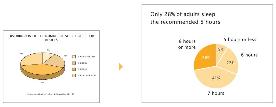
– Here is an example of the usage of figures below. Left one is poorly designed: the title does not point out the key point of the figure, and we can not have a clear idea about the portions. Whilst right one is well designed, clear and simple.


example on figures

An example of the figures in slides from trees maps and theorems, by Jean-luc

Give credit where it is due.
– Making eye contact with the audiences.
– If you do not understand the questions, ask them again first and put off answering them if you really don’t know the answer (for saving time…).